Clustering on the write path

Introduction

Users of lakehouses often fail to realize the impact of ignoring data layout. Sometimes it is the small files induced by the rate of data ingestion; other times it is just blindly applying accepted approaches like partitioning, which also induces small files and unbalanced data layouts.

At Qbeast, we develop indexing and clustering techniques to enable accelerated lakehouse data layouts. We aim to be both table-format- and query-engine-agnostic, without strictly requiring changes to queries. To be clear: our methods require no changes to queries, but in practice, when we examine a customer's performance profile, we repeatedly find issues in their queries that are worth fixing. As we find such problems, we propose query changes, but this is again not required by our methods. We exploit mechanisms such as data pruning and other common query optimizations to benefit from an accelerated data layout.

As part of an accelerated data layout, we have designed our product to enable indexing and clustering as data lands in the table. We aim to be fast enough that landing and optimizing as a second background step become unnecessary, which would otherwise induce write amplification. With Qbeast, the customer can ingest and land new table data in a single step. Indexing and clustering in the write path are not strictly required; a customer can still split into two steps as before if they choose, but we promote having them on the write critical path when suitable because it reduces the write amplification.

The indexing we perform is incremental while being global. Being incremental enables us to reduce the overhead of the additional computation to decide on the clustering. This post is precisely about the speed of indexing and how we envision it being used in the critical write path. We provide performance evaluation numbers that show how efficient our implementation is, comparing it to a baseline and existing implementations.

A recap of Qbeast indexing and clustering

Many expensive queries filter data using multiple columns and might even join tables on those predicates. Multi-dimensional clustering enables efficient filtering and even other query optimizations on operations such as joins and aggregations. To cluster data, we need a technique to determine which records should be grouped together.

Techniques like partitioning achieve this goal, but they are difficult to apply across multiple columns — the number of partitions explodes even with medium cardinality — and they tend to produce an unbalanced file distribution. There are others, such as linear sorting, space-filling curves, and workload-driven clustering. We instead use space partitioning, which avoids the problems we observed with those techniques. Our approach is built on an algorithm we call the OTree: a tree-based index that partitions the multi-dimensional space by locality and data density, built incrementally as data arrives.

We use OTree directly to make clustering decisions: how many files to create per write and which records to put in each file. The index not only enables the expected performance boost when filtering, joining, and aggregating, but also provides an efficient way to obtain representative samples of the data set.

The algorithm works by recursively partitioning the multi-dimensional space into regions called cubes. When a new batch of data arrives, each value in the clustering columns is mapped to a position in the space that determines which cube it belongs to. Every cube has a target row count, and once it reaches the threshold, the overflow spills into child cubes that subdivide its region. Records belonging to the same cube are clustered together and written into the same file. Cubes that do not reach the target are merged bottom-up into their parent or an adjacent sibling to maintain a balanced file size while reducing the impact on min-max intervals.

Since files are immutable in object storage, a file containing data for a given cube can't be reopened to add records to it. Rewriting the affected files on every append would reintroduce the very write amplification and overhead we set out to avoid, so appends never touch existing data. A cube may instead span multiple files with appends as the table grows. We use the term "block" to denote the set of records added to a cube and written to a specific file in a single write operation. This fragmentation into blocks is not permanent, though. Rewrites can still occur during the optimize operation, which compacts the cube blocks and pushes elements to lower levels of the index to rebalance the structure (asynchronously or not).

This block information is saved in the Metadata of the preferred table format (Qbeast can integrate with Delta, Iceberg, or Hudi) and committed using the format protocol. The updated index lives there, and its structure can be rebuilt directly on each new append, allowing incremental clustering of the data.

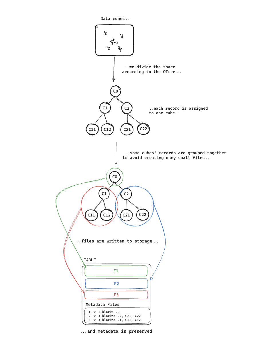
These design choices allow Qbeast to evolve the layout without rewriting existing data. The practical consequence is that the layout is already optimized by the time a query runs. No background job, no deferred cost.

Why clustering on the write path matters

There are two goals worth keeping in mind when effectively organizing the data. First, it is desirable to avoid write amplification, as it affects performance. If we defer clustering to a second step, the data is rewritten each time the operation runs (the original files stick around until they're vacuumed). Second, you want queries to benefit immediately from the layout when you add new data. An efficient layout should make global clustering decisions and shape the files accordingly without requiring a large reorganization.

Qbeast is designed to satisfy both goals at once: it creates a global layout without needing to rewrite any existing files or use two-step clustering (such as Z-ordering, which requires the full data distribution to map values onto the curve). Our goal is to minimize the write overhead by providing a single-step clustering while maintaining incremental properties. That said, if the user workflow is such that it does not require clustering on landing, e.g., a bronze layer that is never or rarely directly queried, Qbeast can also organize the data in separate phases, yielding the same benefits as the single-step path.

In our results section, we aim to put numbers to this argument by evaluating the scalability and efficiency of clustering with Qbeast compared with existing techniques that require data rewriting.

Results

In this post, we argue that clustering should be embedded in the write path and that Qbeast's techniques make it cost-effective to keep it there. For that reason, we measure clustering performance across two scenarios: a real cybersecurity use case with a heavy, deeply nested schema and a TPC-DS fact table. Concretely, we set out to answer some of the following questions:

1. What is the overhead of clustering data using indexing?
2. How does it compare to other clustering techniques?
3. What is the impact of appending data and clustering it after?
4. How does indexing perform with tuning parameters? (Increasing clustering columns, different target row count per cube)
5. How does indexing scale with data volume?

Set up

We ran all experiments on AWS with the following:

• Delta Lake for the table format, version 4.0.1
• Spark 4.0.1
• 4 cores and 25 GB of RAM for the Spark driver
• 4 executors, each with either 4 or 2 cores and 10 GB of RAM (dynamic allocation disabled)
• On-demand m6gd.4xlarge EC2 instances with 950 GB of NVMe disk

For the horizontal scaling evaluation, specifically, we add executors while keeping the same executor configuration (4 cores / 10 GB) unchanged. Each experiment was run three times after a warm-up pass; we report the averages to minimize the impact of outliers and noise.

Clustering comparison

To compare the performance of plain writes (no extra processing) with other existing clustering techniques (e.g., Z-Order), we used a customer dataset on the Cybersecurity Industry. They analyze web pages for potential threats, including phishing, malware, and browser-borne vulnerabilities.

We used a portion of its data to compare Qbeast's write time with other clustering alternatives, such as Z-Order.

• Size in bytes: 97GB (compressed)
• Size in records: ~3M records
• Average row size: ~35,589 kB (compressed)
• Schema: the dataset's columns consist of nested structs and arrays whose sizes vary across rows.

Based on the access pattern to the table, we chose to cluster the web page domain (a String column) and the submission timestamp (as a Long) of the ingested record.

For this and the remaining experiments, we measured the Spark executor runtime, which is the total time a worker node spends actively processing a task, including both CPU compute time and the time required to fetch shuffle data.

The plot compares four executions, each one from a different write technique:

• unclustered — Plain Delta: no clustering, no indexing
• qbeast — Qbeast, clustered directly on append (the default)
• qbeast-clusterAfterAppend — Qbeast, clustered in a separate step after append
• zorder — Delta with Z-order, using the same dimensions as Qbeast

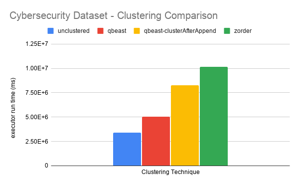
Unclustered is the fastest path for quick ingestion, as expected: it runs no stages beyond the write itself. Qbeast follows, adding ~48% over unclustered while still completing in almost half the time of Zorder. Even if Qbeast indexes and clusters in a second step, it still outperforms Zorder.

Index tuning

There are two main parameters that shape the Qbeast Layout: the columns used for indexing and clustering, and the target row count per file. Depending on how a user configures them, the clustering creates narrow or wide file min-max intervals, changing the final state of the layout. A natural question that arises with this configuration is how this selection affects the performance of the write process.

We used the TPC-DS Store Sales table (SF 1000) for this evaluation. The table characteristics are the following:

• Size in bytes: ~137GB (compressed)
• Size in records: ~3B records
• Average row size: ~56 bytes (compressed)
• Schema: 23 columns, most of them numeric

As a baseline, we choose to cluster two numeric dimensions: the ticket identifier (ss_ticket_number) and the sale price (ss_sales_price). Both are high-cardinality columns, which makes them a good fit for multidimensional clustering.

Tuning row count per file

We used different row counts per file target (100K, 500K, 1M, and 5M) and measured the executor runtime for each experiment.

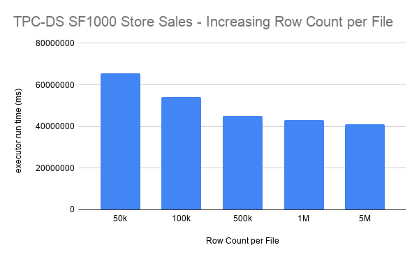
A smaller row count results in a deeper index tree and narrower min-max files. The trade-off is the number of files and the size of the index: we need to process more cubes during writing, and clustering ends up creating more files.

For a 4-executors x 4-cores cluster, the elapsed time stabilizes at around 1M/5M when fewer than 10K cubes are created during indexing.

Tuning clustering columns

The choice of clustering columns determines how many regions the space is split into during indexing, grouping similar values together along each dimension. Choosing columns that appear together in query workloads improves selectivity during searches, since records with similar values across all of them end up in the same file.

Using the same Store Sales table from TPC-DS SF1000, we vary the number of columns clustered while keeping the row count per file fixed at 1M.

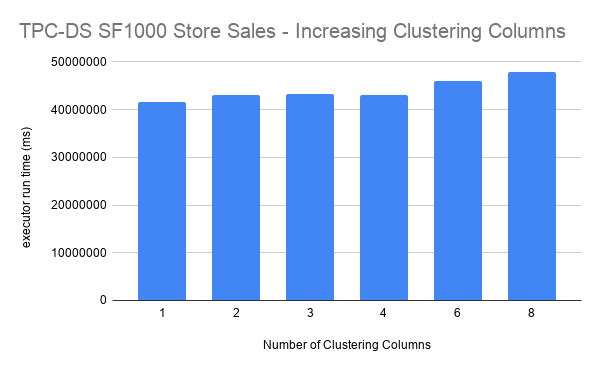
Increasing the number of clustering columns has a small impact: elapsed time rises only about 16% from 1 to 8 columns and does not grow at anywhere near the pace of the target row count parameter.

When we increase the number of clustering columns, the index grows horizontally rather than vertically. With d dimensions, each cube is split into 2^d new regions, so it gets wider and shallower (smaller height). More dimensions don't force more levels; they instead widen each one.

Scalability

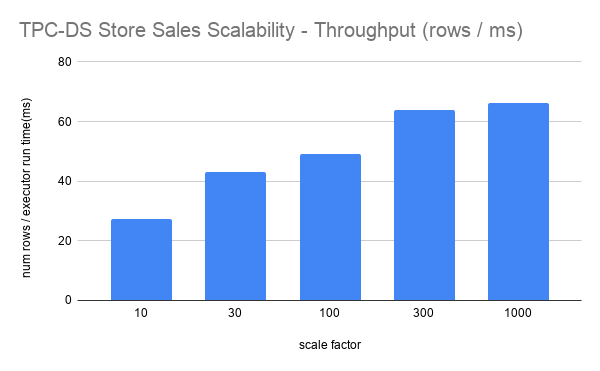
We measured how clustering speed changes with data volume using the TPC-DS Store Sales Table. Because TPC-DS ships with different scale factors, we clustered the datasets ranging from SF10 to SF1000 and captured several metrics, including CPU usage, executor time, and total elapsed time.

Results with fixed cluster

With a fixed cluster size, throughput scales linearly for SF10-SF300, then saturates at ~1M rows/s on SF300-SF1000. This plateau is CPU saturation. On SF300+, the cluster's CPU utilization is ~88–90%, while GC (~0.5%) remains negligible. Once every core is busy, a fixed cluster processes rows at a constant maximum rate, and bigger data workloads take proportionally longer. This raises the following question: is ~1M rows/s a limit of Qbeast, or of the cluster?

Results with scaling executors

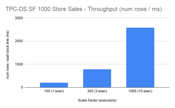
We scaled the number of executors in proportion to the data, holding the work per core roughly constant at ~70M rows/core (1 executor at SF100, 3 at SF300, 10 at SF1000). In this plot, we measured total wall-clock time rather than executor runtime, since we are scaling the number of executors.

From SF100 to SF1000, throughput scales linearly with the added cores. From ~765K rows/s at 12 cores (3 exec) to 2.5M rows/s at 40 cores (10 exec).

Conclusions

This post evaluated the performance of Qbeast clustering on the write path. Some highlights from the results are the following:

• The additional overhead of clustering on write is low compared with other techniques. Indexing with Qbeast completes in half the time compared with Delta Zorder and adds ~48% overhead compared with unclustered Delta.
• Tuning row count per file matters. Adding clustering columns induces a low overhead (~16% from 1 to 8). The one parameter to choose carefully is the target row count per file: a small target forces a deeper tree, an explosion of small files, and longer executor runtime.
• The implementation scales with data volume. On a fixed cluster, indexing throughput grows with data and then saturates at the cluster's CPU ceiling. When we scale the cluster based on the data, indexing time remains roughly constant, and throughput grows linearly, reaching ~2.5M rows/s at 40 cores.

As lakehouse tables often accommodate regularly ingested data from various sources, it is frequently desirable for data to be clustered when committed to the table rather than during an optimize rewrite. We have argued here that Qbeast incurs lower overhead for clustering on write and that it can cluster data as it is written. Our implementation also scales with data volume, satisfying a variety of use-case requirements.